ZIPLINE DESIGN CALCULATION (ANALYSIS)

 

Zipline represents a system where the anchoring points of carrying rope are at different heights, along which the trolley carrying a person is moving. Their original purpose was bridging of canyon or river, often only for lowering the cargo, while today they are more used for the purpose of entertainment as the so- called adrenaline sport.

As it is a relatively new system, whose name has not settled yet, beside the mentioned zipline (which will be used in this paper), it is also known under the names such as: aerial runway, aerial rope slide, death slide or flying fox in English, Seilrutsche in German, Tirolienne in French or Guerillarutsche in the Austrian.

They expanded over the past two decades, with construction in various locations such as hilly areas, parks, lakes, bridges, the city core, etc. Ziplines are mainly foreseen for individual lowering of persons, but there are few cases of ziplines where several persons are lowering side by side (never one behind other). Figure 1 shows an example of parallel zipline located in hilly area. 

FUNDAMENTALS FOR ANALYSIS

This chapter shows a short review of significant relations for the theory of so-called “horizontal rope”, which was developed for calculations of ropeways, cable cranes, overhead power lines, etc. More detailed can be seen in[2], [9] and [10]. 

 

FIG : ZI

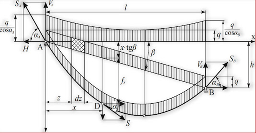
Figure 2 shows a zipline scheme with basic notations. –Rope loaded by its own weight. Line that describes the position of the elastic flexible thread freely hanging between two supports located on the horizontal (l) and vertical (h) distance and loaded with its own weight is called a catenary. The catenary equation can be obtained by observing the static equilibrium of forces shown in Figure 4. 

 

 

Based on the static equilibrium equations that can be written for the elementary section of the rope, and after their rearrangement, the catenary equation is obtained as: 

y=C.cosh(x/C)                                 ….(1)

where the catenary parameter can be defined as:

C=H/q

where: 

• • H – horizontal component of tension rope force, 

• • q – own weight of rope.

The difference of forces between any two points of rope can be determined by the expression: 

∆S= Sb-Sa =q(Ya-Yb ) =q*h                                  ….(2)

The use of catenary theory provides the correct solutions, but as the use of hyperbolic functions is relatively complicated, in the engineering practice the catenary is replaced by the appropriate parabola.

Figure 4 shows the possibility of replacing the catenary with a parabola. The errors in the size of the deflections which are made by this approximation are 2 ÷ 3% (the deflections are smaller in case of parabola than in the case of a catenary). Accuracy can be increased by introducing a correction coefficient (k). 

 

 

Parabola method, obtains the equation of the curve as:

 

where, fx represent deflection which is calculated as:

 

Where:

Rope loaded by its own weight and concentrated load.

Unlike most metal constructions like beams, frames or grids, where the influence of deformation on the static equilibrium is neglected, that is not the case for the “horizontal rope”, so the second-order theory must be applied.  

 

Observing the rope, whose supports are at different heights, which is loaded with its own weight and concentrated load (Q), the equation of the load trajectory, shown on Figure 5, can be presented as: 

y= x*tgβ+fx                     ………..(5)

 where the deflection at the distance XD where the load is acting can be calculated as: 

while the maximal deflection is calculated by :

ANCHORING ROPE ENDS

There are two ways to achieve anchorage of the rope ends:

• • Both side anchorage

• • Anchorage at one end and tightening with the weight at the other.

Figure 6: The rope force change in case of a both sided anchored rope (a) and in the case of tightening with a weight (b)

The case of a both-sided anchored rope is a statically indeterminate system with a significant change in the rope force when the load is moving. Besides that, there is significant impact of temperature and rope elasticity. On the contrary, this case is easy to perform, which is reason why it is often applied for short ziplines (so-called “from tree to tree”). The case of a rope that is anchored at one and tightened with weight at other end is considerably more favorable, because the rope forces aren’t changing much and there aren’t influences of the temperature and rope elasticity, but the system is more expensive, and solution requires more space on the pillar. Change of rope force for three characteristic load positions are notable in Figure 6.

This post will further be based only on the case of rope anchored at one and tensioned with weight at other end.

COMPUTATIONAL MODEL FORMING

The adequate computational model will be formed by neglecting small quantities of high order. The terms (5) and (6) determine the so-called static trajectory of movement. In the case of tensioning with weight and “shallow” catenary, according to [9] and [10], the oscillation of the rope in the vertical plane is relatively small and can be neglected. A person connected with trolley forms a mathematical pendulum, but if the start is smooth and the belt length is short, the effect of swinging can also be ignored. According to that, the computational model, which is shown on Figure 7, can be represented as the concentrated mass that is moving along trajectory determined for static conditions, [5]. Air resistance and rolling resistance are acting onto concentrated mass during the movement, [1], [5] and [13]. The direction of resistances is always opposite to the direction of the movement.

 

As the load is moving along curved path, there is an influence of the centrifugal force. If it is assumed that generally the maximum velocity doesn’t exceed 120 km/h (~33,33 m/s), the maximum possible impact of the centrifugal force in relation to the component of person’s weight is: 

FC_max/Q*cosβ =(Vmax)^2/g*R_min*cosβ 

=(33.33)^2/9.81*4982 ~0.02

where cosβ ~ 1, and the radius of the trajectory curve for given condition is :

R_min= G/(q+2Q/l)

=62500/(10.5+2*1500/1467)

=49820 m

As seen, the maximum impact of the centrifugal force is less than 2%, so it can be ignored.

DERERMINATION OF ROLLING RESISTANCE

Every wheel that is rolling along deformable surface has a resistance component due the friction in wheel bearings and due to deformation of contact surfaces. Wheel that is rolling along the rope has additional resistance component due the rope stiffness. Unlike the perfectly flexible rope, the real rope will not take the position of the tangents behind and in front of the wheel, which can be seen as a “wrinkling” of rope in front of the wheel which is shown on Figure 8. This effect can be included by the relation (8), where the lever arm of rolling torque includes the influence of contact surfaces deformation and the “wrinkling” of the rope, so the value is higher than in case of “standard” wheel. 

 

Resistance of the wheel that is rolling along steel rope is calculated as:

where: 

Based on expression (8) the total resistance coefficient depends on the geometric size of the wheel (d, D), as well as the rolling resistance coefficient in the bearing (μ0) and the rolling resistance between the wheel and rope (f). The bearing friction coefficient and lever arm of rolling torque are determined experimentally.

DETERMINATION OF AIR RESISTANCE

A person travelling along zipline typically generates high velocity, air resistance has a significant impact on all driving parameters. Air resistance is influenced by a large number of dimensions, such as the type of flow (laminar or turbulent), area exposed to the air, the shape of the body, velocity etc. Air resistance is, according to [3], calculated: 

where: 

• • C_w – drag coefficient, 

• • A – frontal area,

• • ρ – air density, 

• • V – person velocity, 

• • Vv – component of wind velocity in the direction of movement, 

• • n – dimensionless exponent depending on velocity, according to [3]: 

• • n=1 for velocities smaller than 1 m/s, 

• • n=2 for velocities between 1 m/s and 300 m/s, 

• • n=3 for velocities greater than 300 m/s. 

As the air density doesn’t change much for some standard conditions, and the velocity is more often expressed in km/h than in m/s, formula (9) can be written in the form:

whereby the velocity (v) is expressed in km/h, the specific air density is taken as ρ=1,225 kg/m3, medium air humidity as w=60% and medium air temperature as t=15 °C.

When temperature or pressure vary from ordinary, a corrected term for density is used: 

where: 

• • B – pressure (bar) 

• • T – temperature (K)

• • The orientationally values of the drag coefficient (C_w) are obtained experimentally and according to [6] approximately amount:

• • – standing person ~0.78,

• • – cyclist in an upright position 0.5–0.69,

• • – cyclist in bent position ~0.4,

COMPUTER SIMULATION 

Within this point the procedure and the results of the analysis for a concrete example of zipline will be presented. Figure 11 shows the geometry of the route with section length of 1467 m and a drop of 99 m. Hence, the inclination angle amounts: 

β= atan (h/l)

= atan (99/1467)

=3.86 degree

This represents a limiting case because of the small inclination angle.

 

The selection of the rope type and its diameter, as well as the foreseen tensile rope force, are detailed elaborated in [12]. The simulation results will be shown for the steel rope of Warrington 6×19+IWRC construction with diameter of 16 mm. Determination of motion parameters was performed using computer simulations in the MSC Adams program package. As mentioned in previous section, the system was modeled as a concentrated mass that moves along a trajectory defined by equation (5). Air and rolling resistance are acting on the concentrated mass which is moving under the influence of its own weight. The direction of resistances is always opposite to the direction of movement. Simulations were performed by varying the person’s weight from 50 to 150 kg. Areas exposed to air depend on the person’s size (weight) and the lowering position, which can be sitting, half-sitting and lying. For case of lowering in a sitting position, those areas can be approximated by the average dimensions of the persons given on Figure 10.

• • A = 0.25 m2 – for persons weighting less than 60 kg,

• • A = 0.3 m2 – for persons weighting between 60 kg and 100 kg,

• • A = 0.4 m2 – for persons weighting between 100 kg and 140 kg,

• • A = 0.5 m2 – for people weighing more than 140 kg. 

 

Areas exposed to air flow for lowering in half-sitting and lying position are smaller and amounts 0.18 m2 and 0.1 m2 respectively.

The drag coefficient depends on the lowering position:

• • Cw = 0.6 – for sitting, 

• • Cw = 0.4 – for the half-sitting and

• • Cw = 0.2 – for lying position. 

The total resistance coefficient of movement, based on the bearing and wheel diameter for concrete trolleys (d = 22 mm and D = 100 mm) and literature-based bearing friction coefficient μ₀ = 0.01 and lever arm of rolling torque f=0.7 mm, is calculated as

µ=µ₀* d/D+2* f/D

=0.01*(22/100) +2*(0.7/100)

=0.016

This average value of the moving resistance coefficient can significantly deviate depending on the d₀/D ratio, bearing type, rope type or H/q ratio. Above mentioned parameters were varied during simulations within limits up to 25%. 

RESULTS OF SIMULATION

Presentation of characteristic result is shown below.

Impact of person’s mass

Diagram of velocity for different values of person’s mass is known on figure11.

 

From Figure 11, it is notable that person do not reach lower station.

-Impact of lowering position The diagram shown on Figure 12 represents the simulation results for the different lowering positions, where it is notable that the seating position cannot be applied for the given conditions

 

However, even the “half-sitting” and “lying” positions should be carefully analyzed, because these positions are significantly more “sensitive” to changes such as spreading of the hand for “selfi” (a larger area), which significantly changes the conditions of the  person’s arrival in the lower station.

–Impact of Wind

Previous paragraphs show only the case of the body moving through the “quiet” air. The following analysis will show the effect of changeable wind direction. The velocity of moderate breeze amounts between 5.5 m/s and 7.9 m/s, so the average values of 6.5 m/s was taken in simulation.

The diagram given on Figure 13 shows the influence of the wind in the direction of movement in the case of the tailwind and headwind for person weighting 50 kg. 

 

BRAKING FORCE DETERMINATION

In the NASA study titled Human Tolerance to Impact Velocities, can be found a diagram shown in Figure 14 that shows the chances of survival when hitting a hard flat surface at different velocities. 

There are three zones on the diagram:

• • zone of certain survival,

• • zone of marginal survival, and

• • fatal zone. 

 

The “zone of certain survival” still carries significant potential for serious injury, so do not mistake that zone as an acceptable, safe, or desirable outcome. 

Knowing that the final speed of the free fall from a certain height is calculated as v =(2*g*h) ^0.5, the diagram given in Figure 15 shows a comparison of arrival velocities to their equivalent free fall distances. These values can be used to assess ziplines arrival speeds and to get an understanding of how far a patron is “falling” when they arrive at a terminal platform. For example, a rider traveling at 30 m/s has the same velocity as someone falling from 45 meters. 

 

The diagram shown in Figure 14 gives information about the possibility of survival when the body moving at a certain speed stops instantly. However, since there is no instantaneous stop at regular usage of zipline, it is much more practical to observe the acceleration or deceleration of passenger. The acceleration or deceleration is manifested by the load on the passenger’s body, so the value of the acceleration will not be observed, but the force that the acceleration, i.e. deceleration, caused. The force is usually not expressed by its intensity but by the relationship to the weight of the passengers, the so-called G-force. Since the human body does not receive a certain G force in all directions equally [15], the coordinate system has been introduced as in Figure 16.

 

According to the ASTM F2291 standard, the maximum value of G-force during braking for sitting. position is allowed in + X direction and has intensity of 6g. However, since the passenger is connected to the trolley by belts which allow swinging in the direction of movement, a braking force of 6g will cause an upward swing and the passenger may hit the zipline cable. It has been empirically determined that the braking force should not exceed the intensity of 2.5g

 

From the equation of work, it follows that the force in the case of stopping a body which was moving at a velocity v on the length l is: 

As already mentioned, the G-force can be defined as the ratio of the force acting on that body and its own weight, so it follows: 

It can be noticed from (13) that the intensity of the G-force, for a certain initial braking velocity, can be influenced by the path, i.e. the length at which the deceleration will take place.

AN EXAMPLE

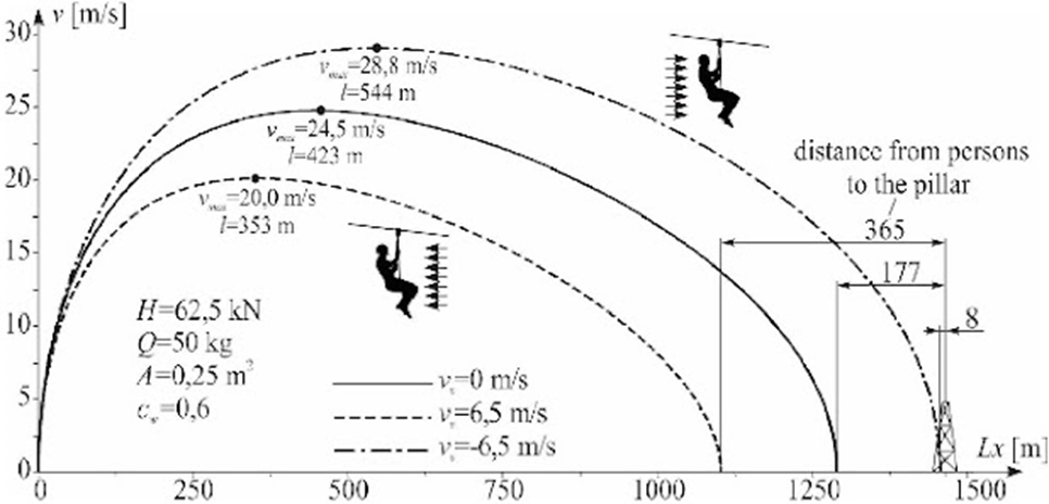
Observing the lowering of a trolley with two passengers in a sitting position (one behind the other) on a concrete zipline a range of 1404 meters, for a case with minimal air and rolling resistances (and thus with maximal velocity), following diagrams of changes in horizontal and vertical velocity components are obtained. 

 

According to the diagram shown in Figure 18, it can be noticed that the horizontal component of velocity at the end of a section has a value of 24.6 m/s and a vertical of 0.5 m/s. Based on that, if there would be an immediate stop, it would be in the zone of marginal survival. Based on (13), if we want to stay in the range up to 6g, a braking distance of: 

Calculation:

l= v²/2*G*g

= (24.6²)/2-6-9.81 =5.1 m is needed

and if we want to stay in the range up to 2.5g, the braking distance should be:

Length= v²/2*G*g

=(24.6)²/2*2.5*9.81

=12.4 m

CONCLUSION

For quality design, production and safe use of zipline, it is necessary to perform a detailed analysis of persons kinematic parameters dependence from a range of influential sizes such as person’s weight, tensile rope force, inclination angle, position during lowering, wheel resistance, wind, etc. It is essential to form an adequate computational model which allows the simulation and determination of so-called “driving characteristics” for concrete conditions.